Origin of Angular Momentum Quantization in Bohr's Model of Hydrogen Atom
Published March 23, 2020
To me, the quantization of angular momentum in the Bohr model of hydrogen has always felt like a very ad hoc assumption. To think that Niels Bohr just happened to come up with the correct quantization condition \(L_z = n \hbar\), (which happens to be identical to what is obtained from a quantum mechanical treatment) is absurd.
Elementary texts explain the quantization rule by appealing to the constructive interference of electron waves (the only orbits permitted are the ones whose circumference is an integral multiple of the de Broglie wavelength of the electron). However, we note that de Broglie formulated his hypothesis more than a decade after the Bohr model was proposed.
In this post, I want to start with the information available to Bohr at the time (evidence for quantized energy levels from atomic spectra and the empirical Rydberg formula) and get to the magical quantization rule with the correspondence principle (as Bohr did).
The following section will start with Bohr’s original postulates and establish some notation, I will discuss the origin of the quantization in the next section.
Bohr’s Postulates
We start with Bohr’s assumptions in his own words:
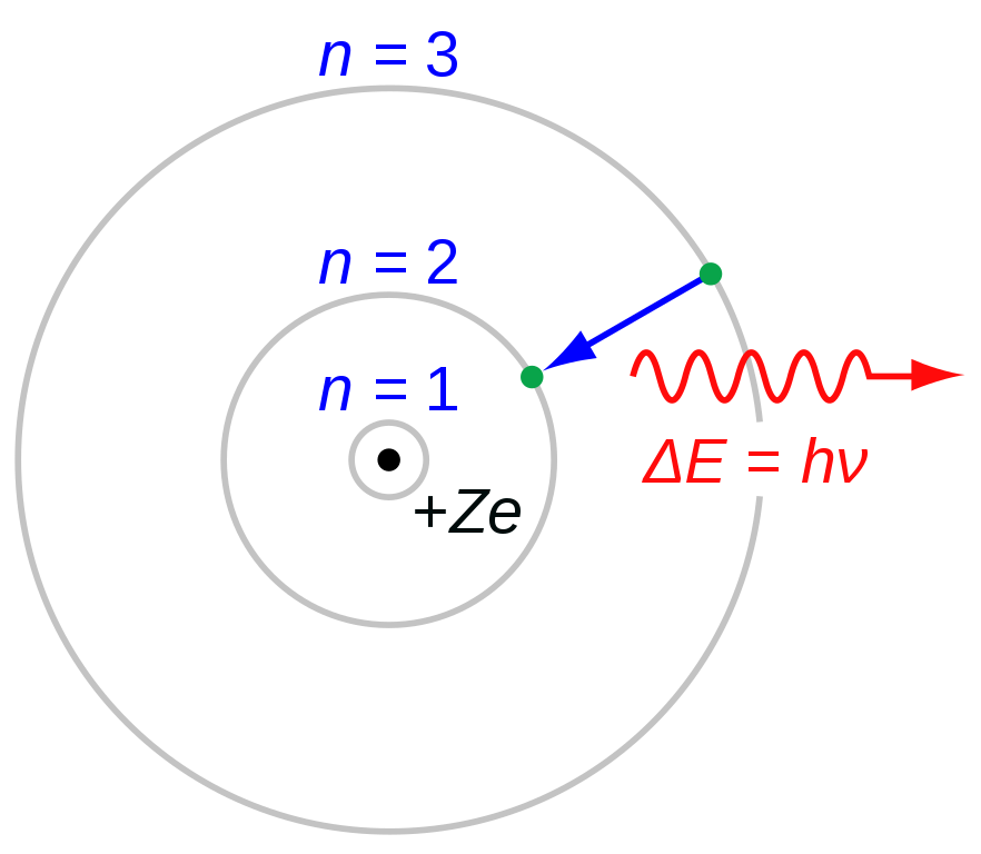
That an atomic system can, and can only, exist permanently in a certain series of states corresponding to a discontinuous series of values for its energy, and that consequently any change of the energy of the system, including emission and absorption of electromagnetic radiation, must take place by a complete transition between two such states. These states will be denoted as the stationary states of the system.
That the radiation absorbed or emitted during a transition between two stationary states is ‘‘unifrequentic’’ and possesses a frequency \(f\), given by the relation \(E' - E'' = hf\), where \(h\) is Planck’s constant and where \(E'\) and \(E''\) are the values of the energy in the two states under consideration.
We note that both of the above assumptions are at odds with classical electrodynamics because (1) accelerating charges radiate away their energy, and electrons in an orbit around the nucleus must be accelerating; and (2) the frequency of radiation given off by a periodically accelerating charge should be the same as the frequency of acceleration.
A third assumption is the corresponence principle which asserts that, as microscopic systems become macroscopic, the results must go over to the classical.
In order to estimate the energy of a stationary state, we equate the Coulomb force on the electron and the centripetal force
\[\frac{e^2}{4 \pi \epsilon_0} \frac{1}{r^2} = \frac{mv^2}{r} \tag{1}\]which leads to the kinetic energy given by
\[T = \frac{1}{2} m v^2 = \frac{1}{2} \frac{e^2}{4 \pi \epsilon_0} \frac{1}{r}. \tag{2}\]The total energy is then given by
\[\begin{align} E & = T + V \\ & = \frac{1}{2} \frac{e^2}{4 \pi \epsilon_0} \frac{1}{r} - \frac{e^2}{4 \pi \epsilon_0} \frac{1}{r} \\ & = - \frac{1}{2} \frac{e^2}{4 \pi \epsilon_0} \frac{1}{r} \tag{3} \end{align}\]We note that the only variable in the above equation is \(r\). Hence if the atomic energy levels are quantized, the atomic radius must also be quantized. Due to the second postulate, frequency of radiation \(f\), emitted due to a transition from energy \(E'\) to \(E''\) (\(E' > E''\)) is given by
\[\begin{align} hf & = E' - E'' \\ & = \frac{1}{2} \frac{e^2}{4 \pi \epsilon_0} \left( \frac{1}{r'} - \frac{1}{r''} \right) \label{e:frequency1} \tag{4} \end{align}\]where \(r'\) and \(r''\) are the atomic radii of the electron in states of energy \(E'\) and \(E''\) respectively. Equation \eqref{e:frequency1}, along with the Rydberg formula
\[\frac{1}{\lambda_{nm}} = R_H \left(\frac{1}{m^2} - \frac{1}{n^2}\right)\\ \label{e:rydberg} \tag{5}\]where \(n\) and \(m\) are integers, and \(R_H\) is a constant referred to as the Rydberg constant which has the units of inverse length, can be used to deduce the quantization of the atomic radii. Since, the frequency and wavelength are related by \(f \lambda = c\), where \(c\) is the speed of light, Equation \eqref{e:rydberg} can be written in terms of the frequency as
\[h f_{nm} = c R_H \left(\frac{1}{m^2} - \frac{1}{n^2}\right) \label{e:rydberg2} \tag{6}\]Expressions in Equations \eqref{e:frequency1} and \eqref{e:rydberg2} lead us to guess that the orbital radii are quantized as
\[r_n = a_0 n^2 \tag{7}\]where \(n\) is an integer and \(a_0\) is a constant with units of length, which for \(n = 1\) gives the radius of the electron orbit in the lowest energy stationary state and is called the Bohr radius.
Now, we need to calculate the Bohr radius. We stop here to note that this is the point when elementary texts ‘assume’ the angular momentum quantization rule, \(L_z = m_e v_n (a_0 n^2) = n \hbar\) as a third postulate to derive an expression for \(a_0\). In this post however, we will use the correspondence principle to derive and expression for \(a_0\) and consequently the quantization rule.
Origin of Angular Momentum Quantization
First, we note that the kinetic energy of the electron is quantized
\[T = \frac{1}{2} m_e v_n^2 = \frac{1}{2} \frac{e^2}{4 \pi \epsilon_0} \frac{1}{a_0 n^2}. \tag{8} \label{e:kinetic}\]Next we recall that, according to classical electrodynamics the frequency of radiation emitted from an oscillating charge is equal to the frequency of oscillation of the charge. According to correspondence principle, the frequency of radiation for transition between adjacent states given by the second postulate, must approach the orbital frequency of the electron in its stationary state for highly energetic states, that is, for large \(r_n\).
The frequency of oscillation of the electron in an orbit of radius \(r_n\) is
\[\begin{equation} f_{orbit} = \frac{v_n}{2 \pi (a_0 n^2)} \label{e:forb} \tag{9} \end{equation}\]Next, we substitute for the velocity from Equation \eqref{e:kinetic}
\[f_{orbit}^2 = \frac{1}{4 \pi^2 n^4 a_0^2} \left[\frac{1}{m_e} \left(\frac{e^2}{4 \pi \epsilon_0}\right) \frac{1}{n^2 a_0}\right] \label{e:forb2} \tag{10}\]The frequency of radiation emitted for transition between adjacent states (between stationary states characterized by \(n\) and \(n + 1\)) can be calculated from the second postulate, and \(f_{radiation}^2\) is given by
\[\begin{align} f_{radiation}^2 & = \left(\frac{1}{2} \left(\frac{e^2}{4 \pi \epsilon_0} \right) \frac{1}{h a_0} \left[\frac{1}{n^2} - \frac{1}{(n + 1)^2}\right] \right)^2 \\ & = \left(\frac{1}{2} \left(\frac{e^2}{4 \pi \epsilon_0} \right) \frac{1}{h a_0} \left[\frac{2n + 1}{n^2 (n + 1)^2} \right] \right)^2. \tag{11} \end{align}\]As \(n\) becomes large, the expression becomes
\[\lim_{n \rightarrow \infty} f_{radiation}^2 = \left[ \left(\frac{e^2}{4 \pi \epsilon_0} \right) \frac{1}{h a_0} \frac{1}{n^3}\right]^2 \tag{12}\]which can be equated to \(f_{orbit}\) and the resulting equation solved for \(a_0\) to obtain
\[a_0 = (4 \pi \epsilon_0) \frac{\hbar^2}{m_e e^2} \tag{13}\]Finally, from Equations \eqref{e:forb} and \eqref{e:forb2}, the velocity of the electron in the \(n\)th Bohr orbit is
\[v_n = \frac{\hbar}{m_e a_0} \frac{1}{n} \tag{14}\]and so the angular momentum is
\[\begin{align} L_z & = m_e v_n r_n \\ & = m_e \left(\frac{\hbar}{m_e a_0} \frac{1}{n}\right) (n^2 a_0) \\ & = n \hbar. \tag{15} \end{align}\]This blog post was inspired by Burkhardt and Leventhal’s treatment of the problem in Topics in Atomic Physics. The primary source, of course, is Bohr’s seminal article titled On the Quantum Theory of Line Spectra.